Our approach to signal source localization uses a particle filter, which is relatively common for a source localization problem. Our specific particle filtering approach derives from Chapter 3 of [1] and uses a generalized likelihood function to account for parameters of RF source which are not known but are assumed to have bounded values.
The use of Unmanned Aerial Systems, UAS, as mobile sensors for RF source localization has been and continues to be explored [2, 3, 4, 5]. A literature review that we recommend may be found in [6]. The work that we present differs from existing methods in three significant ways: 1) We do not rely on directional antennas or known RF parameters; 2) We localize multiple RF sources using real hardware; 3) We use only a Raspberry Pi Zero 2W for sensing.
We assume the use of a multirotor platform carrying a sensor capable of obtaining received signal strength indicator (RSSI) measurements. The position of the multirotor is known and accessible. The algorithm uses only RSSI measurements and their associated locations. The RSSI sensor has been the onboard Wi-Fi of a Raspberry Pi Zero 2W (Pi 2). While this is not an optimal sensor, it demonstrates that specialized hardware is not required.
The Pi2 is a low-cost and low-swap single-board computer capable of running a Linux operating system. The Pi2s that we use run a 64-bit headless version of a Raspberry Pi OS.
We use the Linux IW command-line utility to obtain RSSI measurements using the default Wi-Fi interface WLAN0. The command in 2.1 will produce a list of available Wi-Fi networks, their SSID, their BSSID, and signal strength in dBm. Example output is shown in Appendix A.
$ sudo iw dev wlan0 scan
Upon completing a scan, the RSSI, SSID, and BSSID are collected and written to a file with the latitude, longitude, and altitude of the multirotor platform. We also record the number of GPS satellites to facilitate filtering any measurements with four-position estimates. An example of data recorded in this manner is given in Appendix B. Data is formatted as described in the table below.
| Column | 1 | 2 | 3 | 4 | 5 | 6 | 7 |
|---|---|---|---|---|---|---|---|
| Content | SSID | RSSI | BSSID | latitude (°) | longitude (°) | altitude (m AGL) | GPS satellites |
Table 1: Description of data
Note, the Pi 2 onboard Wi-Fi only support 2.4 GHz bands. As a result, active scanning uses IW is faster on the Pi 2 than it would be with other devices that also scan 5 GHz bands. As implemented, our Pi 2 is able to scan at a rate faster than 1 Hz. To date, we have not attempted running localization online on the Pi 2. Localization has been accomplished in post-processing by polling the data file generated by the Pi 2. We also know that passive scanning may be accomplished using devices that support promiscuous mode. We have not explored that option.
Our specific particle filtering approach derives from chapter [3] of [1]. Specifically the RSSI measurement in dB is assumed to be represented by the model
where is the received power (in decibels) at a short reference distance
from the source,
is the propagation loss from the source to the sensor,
is the Euclidean distance from the source to the sensor (in meters), and
is zero-mean Gaussian white noise with known standard deviation
.
Ideally, the propagation loss in free space is 2. However,
will be distinct at different locations due to multipath and shadowing. In some applications, it is desirable to learn
as a function of sensor and source location. We won't be able to do that, so we just need to deal with the uncertainty. In practice,
is between 2 and 4. We do not have access to the reference power
of the source that we're localizing. We assume that
.
Our approach to localization (described in Chapter 3 of [1]) is to use a particle filter. Each particle in our filter represents a hypothesis of the radio parameters and a position
that gives a distance when compared to the location where a measurement is taken,
. Using the generalized likelihood function in [1], we evaluate the likelihood of each hypothesis for each new measurement. The least likely hypotheses are discarded and replaced with new hypotheses. Over time, hypotheses that are not supported by the data are culled, and the surviving hypotheses (particles) give a probability distribution over the possible position of the true RF source.
Experiments were performed by placing wifi routers at known locations and having a survey device pass by in an ad-hoc search pattern. The data obtained during the flight were pulled from the survey device and the particle filter localization algorithm was run on a separate laptop computer for each wfif network recorded in the data. Results from a single survey performed at an undisclosed location.
Figure 1 shows the search pattern that surveyed. Visualization is accomplished using the python folium package.
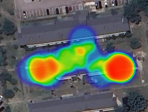
Figure 1