iRamat

Tools for archaeometry and archaeometallurgy in R

---

Install from GitHub

# installinstall.packages("devtools")
devtools::install_github("iramat/iRamat")

Load the iRamat package

library(iRamat)

Using the Database API

Connect the database API with the default parameters, and show the first row, using the db_api_connect() function

df <- db_api_connect()

The default dataset is dataset_adisser17

names(df)
# [1] "dataset_adisser17"

The dataset can by accessed by its name:

head(df$dataset_adisser17, 2)

site_name	id_chips	sample_name	typology	na	mg	al	si	p	s	cl	k	ca	mn	fe	loi	ag	arsenic	ba	be	bi	cd	ce	co	cr	cs	cu	dy	er	eu	deltafe56	deltafe57	ga	gd	ge	hf	ho	indium	la	li	lu	mo	nb	nd	ni	os	os187_os188	os187_os186	pb	pd	pr	rb	ru	sb	sc	se	sm	sn	sr	sr87_sr86	ta	tb	te	th	ti	tl	tm	u	v	w	y	yb	zn	zr	major_method	major_analytical_setup	trace_method	trace_analytical_setup	reference	url
Aux Minières	4967	MINHAO108-A	NA	0.04	0.03	3.23	4.45	0.04	0.00	0	0.07	0.09	0.03	53.17	7.90	NA	578.900	20.31	13.500	0.308	0.325	56.06	26.590	214.9	0.971	5.587	5.025	2.637	1.387	NA	NA	7.478	4.960	2.61	1.431	0.938	0.475	21.24	NA	0.372	5.362	2.808	24.37	63.140	NA	NA	NA	113.8444	NA	6.119	4.692	NA	127.50	1.342	NA	6.095	0.945	43.73	NA	0.227	0.843	NA	17.38	0.092	NA	0.397	9.352	857.3	0.563	22.17	2.776	112.60	58.04	ICP-OES	CRPG - Thermo Fisher Scientific Icap 6500	ICP-OES	CRPG - Thermo Fisher Scientific Icap 6500	Alexandre Disser, Philippe Dillmann, Marc Leroy, Maxime L'Héritier, Sylvain Bauvais, Philippe Fluzin (2017), Iron Supply for the Building of Metz Cathedral: New Methodological Development for Provenance Studies and Historical Considerations, Archaeometry, 59	https://onlinelibrary.wiley.com/doi/full/10.1111/arcm.12265

Chronology

Site timelines

The chrono() function models the chronological attribution of the site by creating a timeline:

df <- db_api_connect()
chrono(d = df$dataset_adisser17)

PeriodO timelines

PeriodO periods can also be displayed. The default Periodo authority (i.e. a set of different periods identified by the same author) is INRAP: Institut National de Recherches Archeologiques Preventive.

periodo(min_date = -700, max_date = 0, use_periodo = TRUE, time_match = 1)

Sites and PeriodO timelines

Site and PeriodO timelines can be merged into a single plot:

df <- db_api_connect()
plots <- chrono(df$dataset_adisser17, use_periodo = TRUE)
ggpubr::ggarrange(plots$sites, plots$periodo$periodo,
                  heights = c(1, 2), ncol = 1, align = "v")

Point Pattern and spatial analysis

Point Pattern Analysis

The ppa() function performs different point pattern analysis (PPA) on raster grids or spatial data. It could be used to assess if a point distribution is regular, clustered or random.

regular	clustered	random

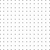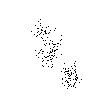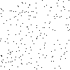Run the function with its default parameters:

d <- ppa()

d is a hash-like object (similar to a Python dictionary) that stores different test outputs: Quadrat test, K-Ripley test, G-function test. Let's call some of these results:

Quadrat test

Check the Quadrat test of the clustered distribution

d[["clustered_distribution.png"]]$quadrat

	Chi-squared test of CSR using quadrat counts

data:  pp
X2 = 732.01, df = 24, p-value < 2.2e-16
alternative hypothesis: two.sided

Quadrats: 5 by 5 grid of tiles

K-Ripley test

plot(d[["clustered_distribution.png"]]$ripley, main = "clustered distribution")

G-function test

plot(d[['regular_distribution.png']]$gfunction, main = "regular distribution")