4. Tutorials
This series of tutorials has been created to introduce the user to VIAMD and its functionalities. Each tutorial introduces new visual and analysis components and highlights the interactivity of VIAMD. For the moment, the tutorial #1 and #2 have been tested by several users. The tutorial #3 and #4 are under construction.
This first tutorial is going to use the preloaded dataset that is automatically loaded when opening VIAMD. It consists of a short trajectory (500 frames) of a single chain consisting of 15 alanine residues.
There is no prerequisite knowledge for this tutorial except a curiosity about molecular dynamics.
- Take some time to get familiar with the navigation in the spatial view. Using the left mouse button, you can rotate the 3D model while holding the right mouse button translates the model. A double click on an atom re-centers the view and sets the camera focus to this specific atom while a double click on the empty background will reset the view.
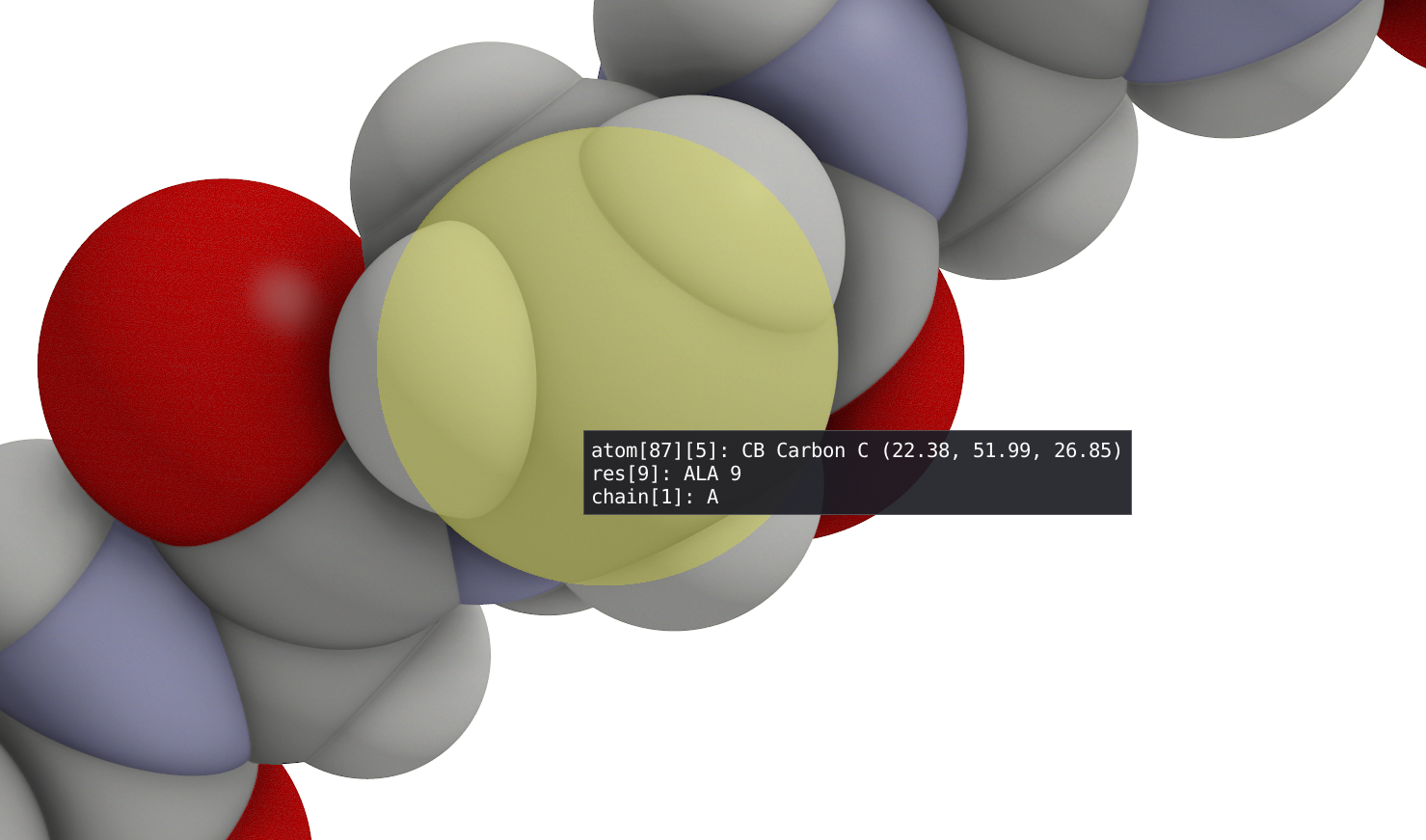
- Hover around atoms to get information. The first line indicates the global atom number, residue atom number, atom type, element as well as xyz coordinates. The second line indicates residue name and residue number. And the last line indicates chain name and number.
In the animation windows, you can start and pause the animation of your trajectory and use the time slider to navigate through it. Alternatively, in the spatial view, you can use the space bar to start and stop the animation.
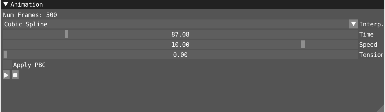
- Use the speed slider to tune the speed of the animation.
- Take some time to experiment with the three interpolation modes provided: nearest, linear, and cubic.
- Take some time to read the lines in the script editor and understand the different properties that are being evaluated.
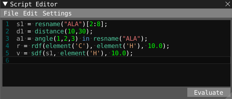
- You can get help through visual feedback by hovering over expressions in the script editor window.
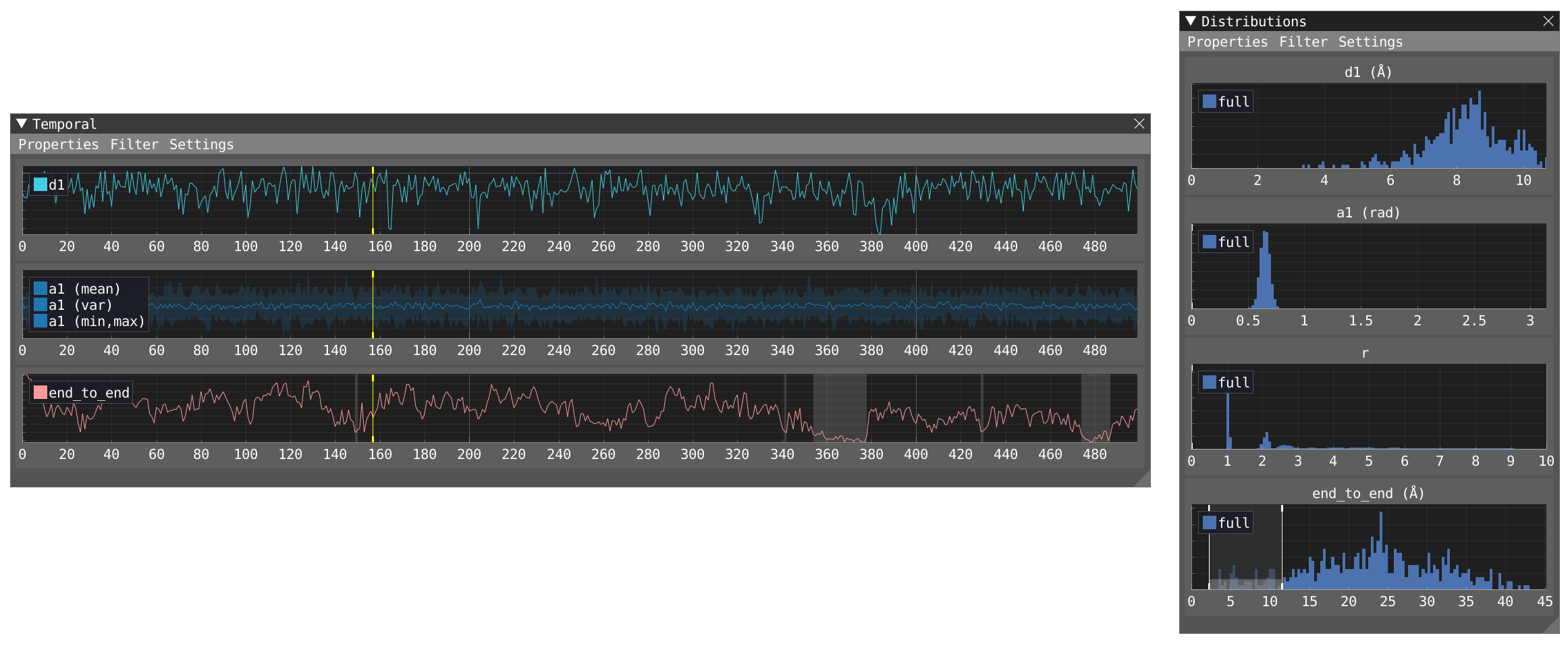
- Click on the evaluate button and open the timeline window. To display properties evaluated, you can click on Properties in the Temporal window and drag and drop the propertie(s) of your choice in the temporal window. Note that you can increase the number of subplots. To navigate on the timeline, you can zoom in and out with the scroll button of your mouse. Once zoomed in, you can drag and navigate your timeline by left clicking and dragging. While pressing the CTRL key and left mouse button, you will jump to this specific point of the trajectory. Double click to reset the view. By hovering on the time line you get a visual feedback of the calculated property in the 3D view.

- Open the distribution window. The functioning is very similar to the Timeline window as you can drag and drop properties in the window. You can plot several distributions on the same plot and/or use different subplots. You can also zoom in and out with the scroll button of your mouse and navigate with a left click and drag. Double click to reset the view. The distribution is also linked to the timeline and by hovering you get visual feedback in the timeline and in the 3D view.

- An easy way to calculate new properties is to type in a new formula and evaluate it. To evaluate the distance between the extremity of the chain (
end_to_end), we can type in the following formula in the script editor. You can find a list of functions available on the language page.
end_to_end = distance(1,151);
-
Another way is by selecting atom(s) in the spatial view by using a left-click of the mouse in combination with the Shift key. To unselect, hold Shift while right-clicking. A right click on the selection opens the context menu. Open the context menu and select Script:
- when two atoms are selected, VIAMD is going to propose you to calculate a distance or save a selection
- when three atoms are selected, VIAMD is going to propose you to calculate an angle or save a selection
- when four atoms are selected, VIAMD is going to propose you to calculate a dihedral angle or save a selection
- when more than four atoms are selected, VIAMD is going to propose you to save it as a selection.
-
Select two atoms at the extremity of the chain (atom 1 and 151) and use the context menu to add the distance expression to the script editor. Rename this new variable
end_to_end. Then, evaluate it.
- Activate the filter in the timeline window and decide the extent of the temporal window. This will add another distribution (filt) for each evaluated parameter in the Distribution window in addition to the distributions of the full trajectory (full). Play the movie and see how it affects the distribution.
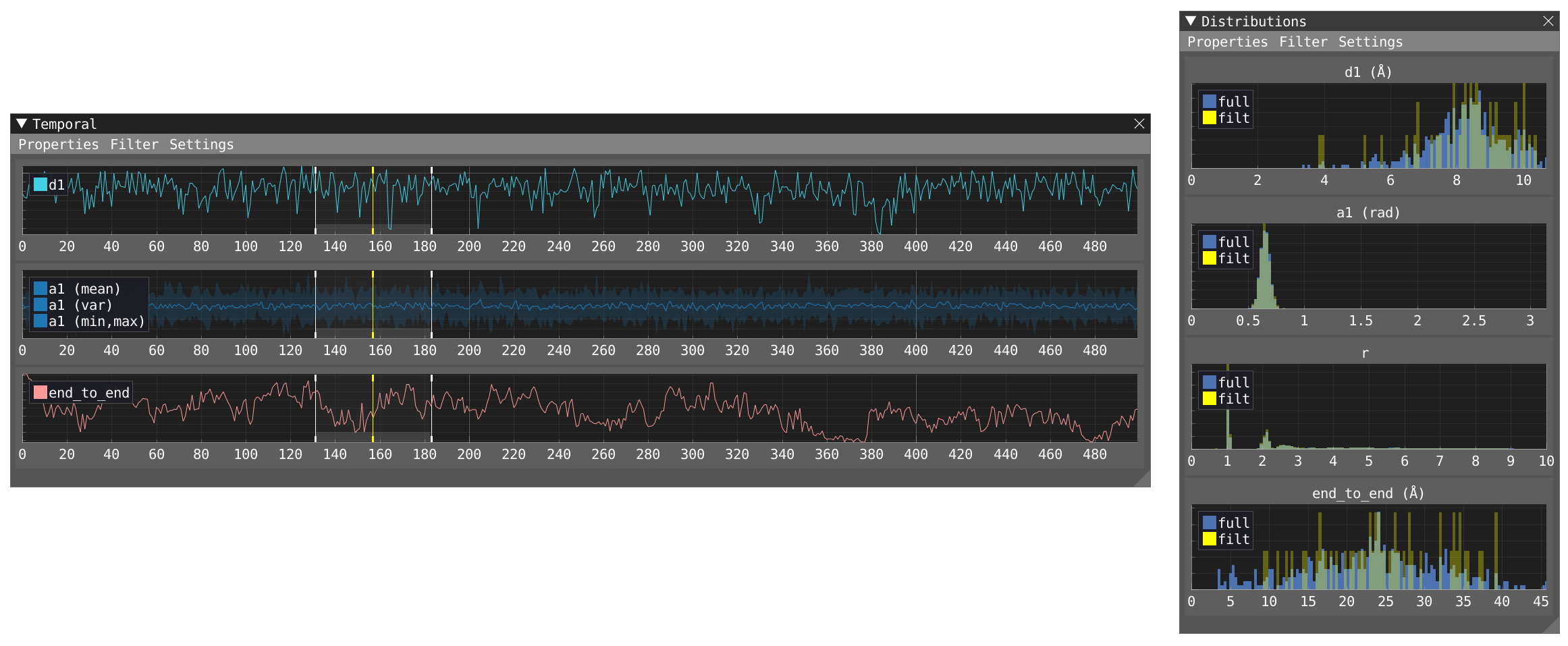
- Activate the filter in the distribution and let's focus on the distribution of the
end_to_enddistance. By dragging the filter at the left of the window you can filter for shortend_to_enddistances. In the timeline, matching areas are highlighted in gray the moment they fall within the filtered distribution.
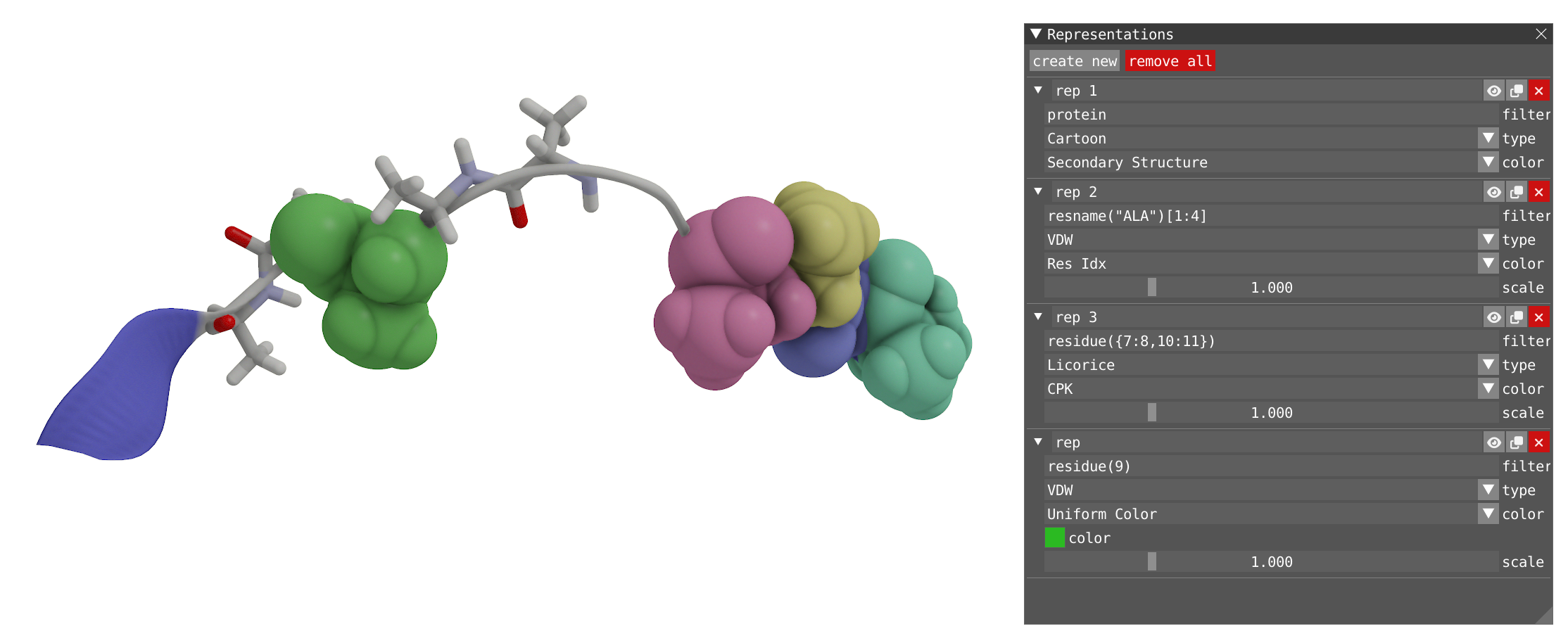
By using the menu Windows -> Representations, you open the representation window where you can create/remove, enabled/disabled, clone, and edit different representations for your system: A representation is comprised of a text-based filter using VIAMD language, which evaluates into an atom visibility mask, a visualization type, and a color scheme.
- Try to modify the current representation and experiment with the type and color. Settle for Cartoon as the type and Secondary structure as coloring to visualize the change between beta-sheet (blue) and alpha-helice (grey).
- Create a new representation. By default the new created representation as no filter (all), you can try to apply a filter and get familiar with the VIAMD language. Here a few examples of filter that can be used:
residue(1:5)
atom(6:90)
resname("ALA")
- Here is an example of several representations using filtering:
- Let's now get back to a single VDW representation and choose property as a color. Choose
end_to_endas a property, as well as your favorite color scale. Then click the auto-update button. Play back the trajectory. The full molecule is now colored in a function of theend_to_enddistance.
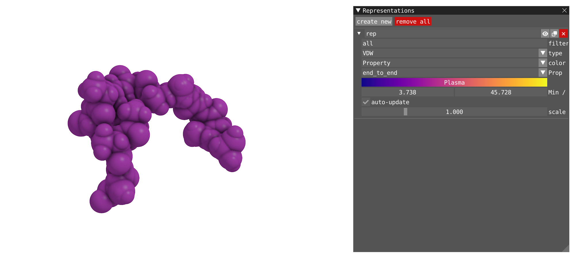
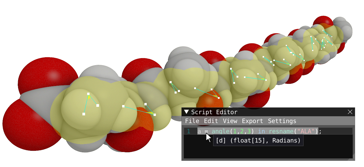
- Now change the property for
a1, the individual atoms1,2and3of each alanine are now colored in a function of the angle between each atom 1, 2 and 3.
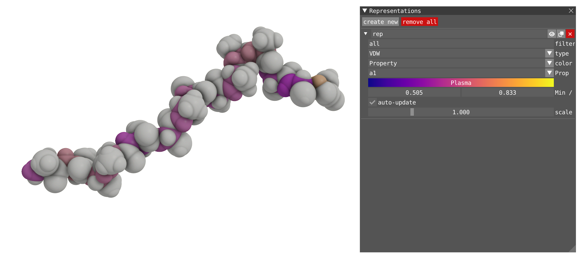
- Note that for the moment, only a single representation can be colored by a property.

This second tutorial is going to use the dataset #2. This dataset consists of an aspirin ligand being pulled out of its specific binding to Phospholipase A2. The dynamic was performed from the crystal structure (1OXR) of the complex. In this dynamic a biased potential was applied to pull the molecule out of pocket. This trajectory has been obtain with GROMACS using the Amber force-field. This trajectory was produce for pedagogical purpose for this tutorial. It is available to download from the provided link. An edr file of the trajectory is also provided.

You are expected to have performed the first tutorial before starting this one.
- By using the menu File -> Load Data, load the file aspirin-phospholipase.gro.
- Then by using the menu File -> Load Data, load the corresponding trajectory file aspirin-phospholipase.xtc.
- Alternatively you can drag and drop the two files successively.
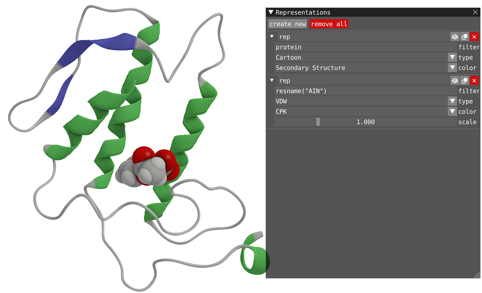
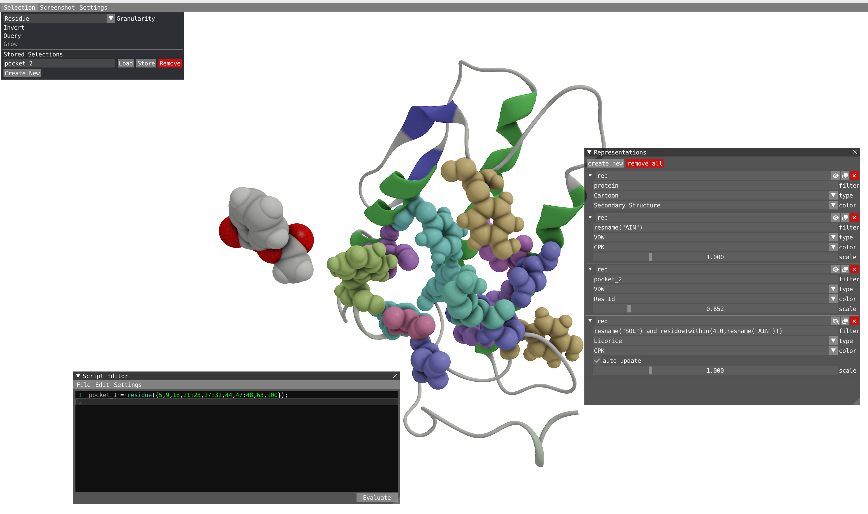
- Open the Representations window and modify to have two representations:
- One for the Protein with Cartoon type and Secondary Structure coloring.
- One for the aspirin (residue name: AIN) with VdW type and CPK coloring.
Reveal to show how your system should look like
- With a right-click of the mouse on the aspirin molecule, you can open the menu and select Recenter Trajectory and then on Residue.
- Play the trajectory.
- Recenter the trajectory on the protein by right-click, select Recenter Trajectory and then on Chain.
- In the Animation window, go at the beginning of the trajectory.
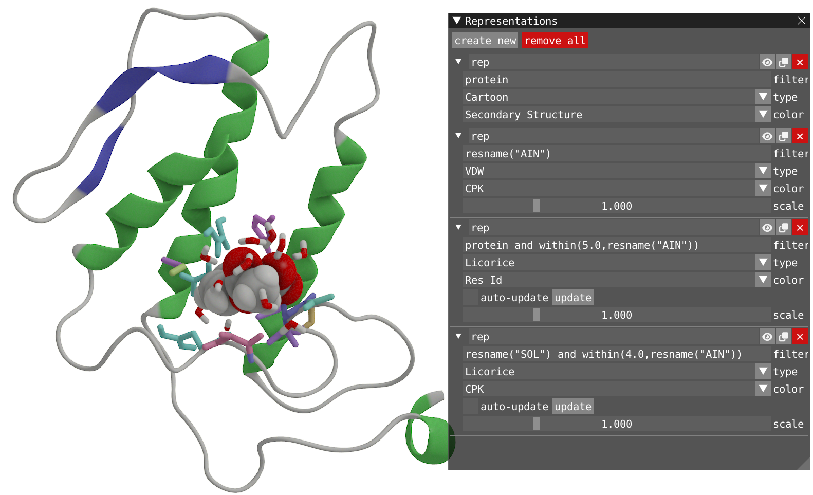
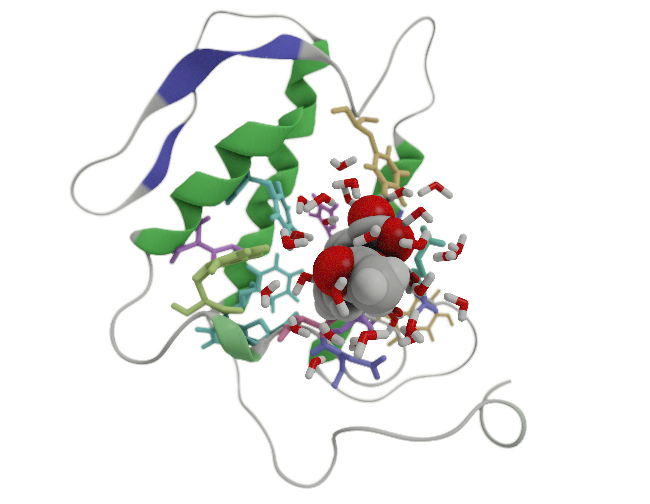
- By using the keyword within, add two new representations:
- One for the atom in the protein within a radius of 5 Å of the residue AIN. Aka, the pocket. This representation should have Licorice type and Res Idx coloring.
- One for the atom of water within in a radius of 4 Å of the residue AIN. This representation should have Licorice type and CPK coloring.
Reveal to show how your system should look like
- Play the dynamic without ticking the two auto-update checkboxes and observe what is happening.
- Go to the beginning of the trajectory.
- Tick the box to auto-update for the representation of water around the aspirin molecule only and play the dynamic. In this way, you keep the representation of the pocket unchanged when the molecule is leaving the pocket, while the water around the aspirin molecule are updated for every frame.
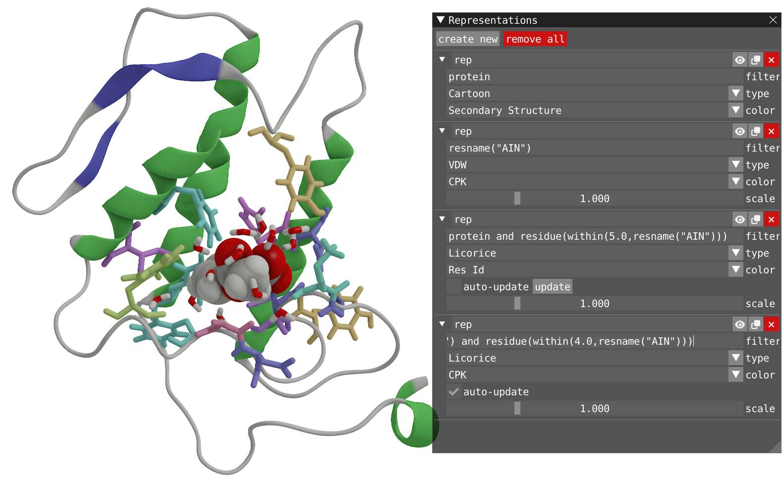
- You can observe that the dynamic selection used so far incorporate the atoms within 5 Å of residue AIN. Try to modify the two expressions used for filtering by using the function 'residue()' to incorporate all the atom of a residue if any atom of this residue is included.
Reveal to show how your system should look like
Take some time to look at the Visual menu, where one can tune several parameters to improve the look of the visualization.
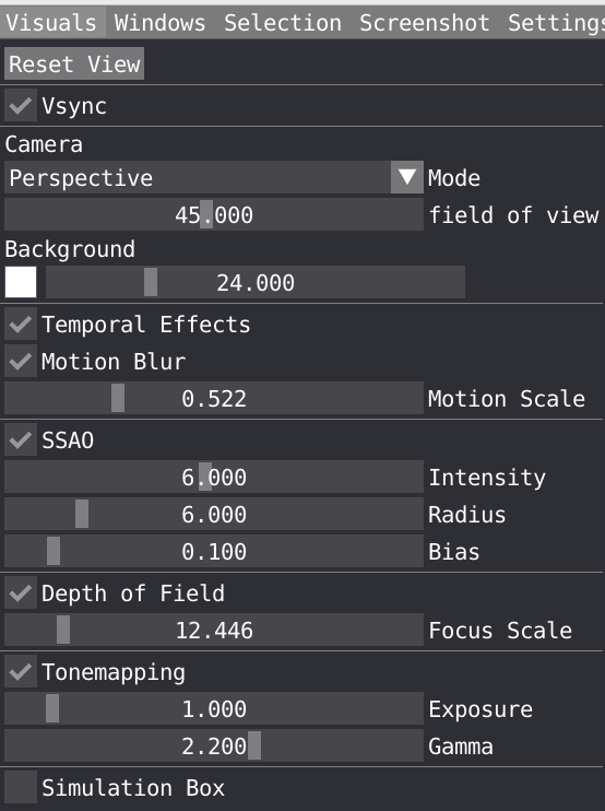
- You can choose Camera mode between Orthographic and Perspective and change the field of view for the latter, you can also change the background color and saturation.
- Temporal effects is a package feature which includes temporal anti-aliasing and optional motion blur.
- You can tune the following Screen Space Ambient Occlusion (SSAO) parameters: Intensity, Radius, Bias. These parameters are important to play with to properly describe shadow in cavity for example.
- Change the Depth of Field to create some blur effect. For that double click on the aspirin molecule to focus the camera on it and adjust the depth of field.
- Tonemapping: VIAMD internally uses an ad-hoc physically based lighting model with photometric units as floating point numbers that needs to be mapped to the display range (0-255). The tonemapper controls performs this operations and can be configured using parameters such as exposure and gamma to control the curve.
- Ticking the box will display the simulation box in the spatial view. You can adjust the width and line color.
Reveal to see if you did a better job than the author of this tutorial to create a beautiful visualization
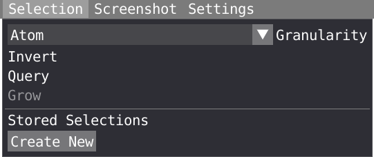
In this part of the tutorial we will use the selection tools to define the binding pocket of the aspirin molecule. In the spatial view, the user can make spatial selections of individual atoms or regions by using a left-click of the mouse in combination with the SHIFT key. To unselect, SHIFT + right-click. With a right-click on the selected region and choosing the Selection menu, you can invert, query or grow your selection.

We are now going the selection tool to select the pocket and save the selection. We are going to do that in two ways
- The first way is going to take profit of the filtering done in the representations:
- Used a VDW representation for the residue of protein within 5.0 Å of the aspirin molecule.
- Set the granularity level to residue in the selection menu.
- In combination with the SHIFT key, left-click on all the residue making the pocket. You can rotate and zoom, as well as move backward and forward to move the aspirin molecule away.
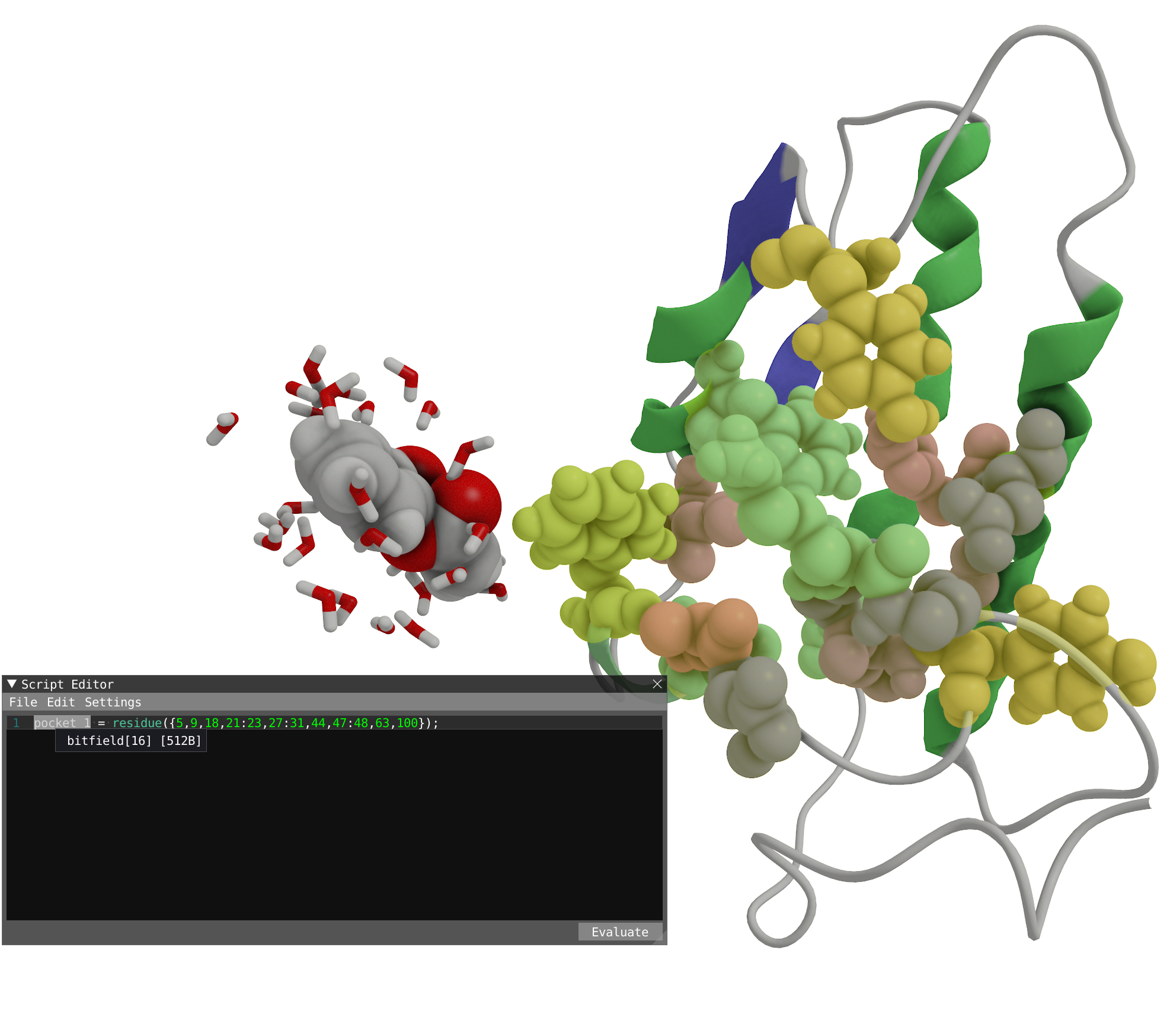
- Do a right-click on your selection and select script, save your selection at the residue level in the script editor.
- Rename your selection as pocket_1 in the script editor
Reveal to see how your system should look like.
Another option
Instead of manually left-clicking on all the residue making the pocket, one could make use of the previous representation to target all the atoms making the pocket:sel1 = residue(protein and within(5.0, resname("AIN")));
- Another way to select the pocket is to use the radial grow tool of the selection:
- Let's start by hiding the water molecule in our representations and go at the beginning of the trajectory.
- Select the aspirin molecule and then right click on it to open the selection menu and choose Grow.
- Choose radial and grow by 5Å and then Apply.
- Remove the aspirin molecule from your selection: SHIFT + right-click on the aspirin.
- In the Selection menu, you can Create a new stored selection.
- Call it pocket_2 and store it.
- Now pocket_2 could be used as a filter for representations or property calculation.
Reveal to show how your system should look like
In this part of the tutorial, we will define some key geometrical parameters to analyze this trajectory.
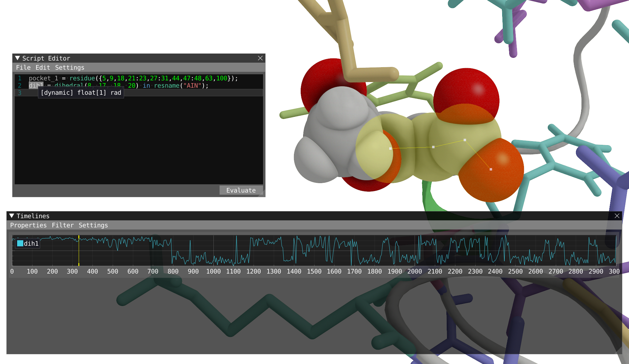
- Let's start by evaluating the dihedral
dih1, dihedral angle by the individual atoms8,17,18, and20of the aspirin molecule:- This can be done directly in the script editor. Note, that if you want to do that by selecting the four atoms in the spatial view, you need first to change the granularity level to atom in the selection menu.
- Evaluate and display the timeline.
Reveal to show how your system should look like
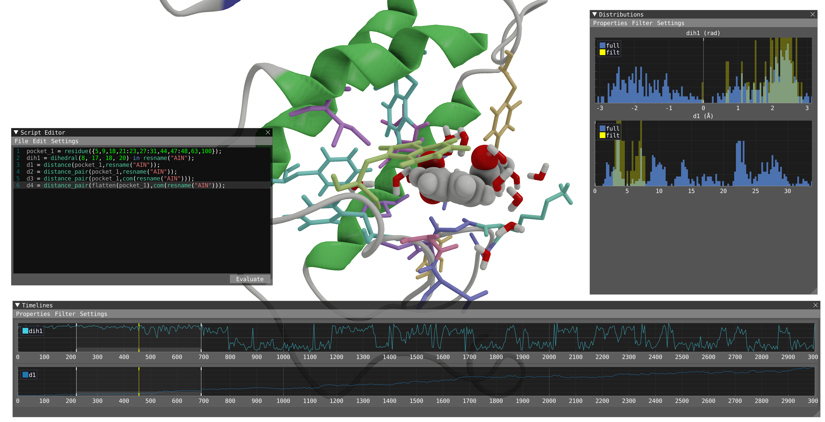
- Let's now focus on calculating the distance between the pocket and the aspirin molecule. A simple way to do that is to use the distance function:
d1 = distance(pocket_1,resname("AIN"));
- Play with the language with trying the different expressions and use visual feedback to understand the difference between the different expression:
d2 = distance_pair(pocket_1,resname("AIN"));
d3 = distance_pair(pocket_1,com(resname("AIN")));
d4 = distance_pair(flatten(pocket_1),com(resname("AIN")));
- Let's know focus on dih1 and d1 only, we recommend to hide the other parameters in the timeline and distribution:
- You can turn on the filtering in the timeline to obtain filtered distribution.
- By looking at both dih1 and d1 properties and playing the dynamic with filtering, we can clearly correlate the change in dih1 to the distance to the pocket. When bound to the protein, the aspirin is locked in a conformation and start to rotate freely after leaving the pocket.
Reveal to show how your system should look like
Import the LJ and Coulombic interaction energies between the protein and the aspirin molecule and sum them as a new property tot.
Reveal to show how your system should look like

Take some time to explore the trajectory with all the properties plotted and filtering to understand how they are connected.
A workspace file (.via) can be saved and will include information regarding your trajectory input file(s) (relative path with respect to via file), the camera position and focus, the different representations used, the content of your VIAMD script editor as well as some rendering information (SSAO,...). This .via file can then be loaded directly in VIAMD (Open Workspace). Alternatively, you can drag and drop a via file in VIAMD for automatic loading.
- Save your workspace.
- Open it with a text editor and text some time to understand the different part.
- You can modify the .via file in a text editor prior to opening in with VIAMD.
This is more or less how your workspace file should look like
[Files] MoleculeFile=aspirin-phospholipase.gro TrajectoryFile=aspirin-phospholipase.xtc CoarseGrained=0 Deperiodize=1[Animation] Frame=91.126 Fps=6.32 Interpolation=2
[RenderSettings] SsaoEnabled=1 SsaoIntensity=10 SsaoRadius=7.146 SsaoBias=0.26 DofEnabled=0 DofFocusScale=1
[Camera] Position=1.80133,21.8221,77.5342 Rotation=0.0953498,-0.465246,0.140921,0.868675 Distance=54.3429
[Representation] Name=rep Filter=protein Enabled=1 Type=3 ColorMapping=8 StaticColor=1,1,1,1 Radius=1 Tension=0.5 Width=1 Thickness=1
[Representation] Name=rep Filter=resname("AIN") Enabled=1 Type=0 ColorMapping=1 StaticColor=1,1,1,1 Radius=0.667 Tension=0.5 Width=1 Thickness=1
[Representation] Name=rep Filter=protein and residue(within(5.0,resname("AIN"))) Enabled=1 Type=1 ColorMapping=4 StaticColor=1,1,1,1 Radius=0.652 Tension=0.5 Width=1 Thickness=1
[Representation] Name=rep Filter=resname("SOL") and residue(within(4.0,resname("AIN"))) Enabled=1 Type=1 ColorMapping=1 StaticColor=1,1,1,1 Radius=1 Tension=0.5 Width=1 Thickness=1
[Script] Text="""pocket_1 = residue({5,9,18,21:23,27:31,44,47:48,63,100}); dih1 = dihedral(8, 17, 18, 20) in resname("AIN"); d1 = distance(pocket_1,resname("AIN")); d2 = distance_pair(pocket_1,resname("AIN")); d3 = distance_pair(pocket_1,com(resname("AIN"))); d4 = distance_pair(flatten(pocket_1),com(resname("AIN"))); edr = import ('aspirin-phospholipase.edr'); Coul = import('aspirin-phospholipase.edr', 67); LJ = import('aspirin-phospholipase.edr', 68); Tot = Coul + LJ; """
[Selection] Label=pocket_2 Mask=###JwMAAAABAAIAgAAC8P8fIAgBwH8gBIAAB/j//wAA4P//YBcgDCAAAAeAGYAAAP5AM+AFEkAAAvD/P0AG4BwAAcD/4AFu4AUAAsD//0Ce4BcABAAAAAAA###
This third tutorial is going to use the dataset #3. This non-biased molecular dynamic simulation illustrates the binding of a pentameric oligothiophene used for the detection of amyloid-β(1–42), responsible for Alzheimer’s disease. It is available to download from the provided link.

You are expected to have performed the first and second tutorial before starting this one.
- By using the menu File -> Load Data, load the file amyloid-pftaa.gro
- Then by using the menu File -> Load Data, load the corresponding trajectory file amyloid-pftaa.xtc
- Open the Representations window and modify to have two representations:
- One for the Protein with Cartoon type and Secondary Structure coloring.
- One for the PFTAA molecules, aks probes (residue name: PFT) with VdW type and CPK coloring.
Reveal to show how your system should look like

- We can start by counting the number of residue PFT attached to the amyloid fibrils during the trajectory. You can use the count and within function to select all the probes within 2.0 Å of the protein and then evaluate.
Reveal to show how your system should look like

-
By hovering on the time line, you can see the number of molecules attached to the fibrils along the trajectory. This operation being computationally intense, we recommend you to comment this line for the rest of the tutorial.
-
We are then going to select a subset of probes that are adsorbed during the full trajectory. For that place yourself at the first step of the simulation and use the Selection Query to select all the PFT residues within 2.0 Å of the protein. Apply and save your selection by right clicking one of the highlighted molecules. Name your selection "ads" in the script and evaluate it.
Reveal to show how your system should look like

- To check that all the molecules in the ads subset stay adsorbed during the full trajectory. You can define new representation using the "ads" filter and coloring the molecules in red for instance, You need to increase slightly the vdw radius of the representation. By playing the trajectory, you can make sure than all the red molecules stay adsorbed.
Reveal to show how your system should look like

-
To define a subset of molecules not adsorbed to the protein, we are going to place ourselves at the end of the trajectory and using the same Selection Query as before, select all the molecules adsorbed and save them as "ads_end". You can then create a "not_ads" group by excluding the "ads_end group and the protein. You can then evaluate.
-
To define a subset of molecules not adsorbed to the protein, we are going to place ourselves at the end of the trajectory and using the same Selection Query as before, select all the molecules adsorbed and save them as "ads_end". You can then create a "not_ads" group by excluding the "ads_end" group and the protein. You can then evaluate.
-
To check that all the molecules in the not_ads subset are not adsorbed during the full trajectory. You can define a new representation using the "not_ads" filter and coloring the molecules in green for instance, You need to increase slightly the vdw radius of the representation. By playing the trajectory, you can make sure than all the green molecules are never adsorbed during the trajectory.
Reveal to show how your system should look like

- For the full trajectory Zoom in on a PFT molecules and select (SHIFT + left-click) the fours atoms 22, 20, 1, 2. Then right click on the selection and then click on Script. Choose then to calculate the dihedral angle for resname("PFT"). dih1 will appear in your script editor.
Reveal to show how your system should look like

Reveal to show how your system should look like

- We can then repeat the operation but instead calculating the distributions only for the molecule adsorbed during the trajectory. For that we can just define a new parameters dih(i)-ads by applying the calculation of the dihedral only to the "ads" subset. Once done, you can then evaluate.
Reveal to show how your system should look like

- We can repeat the same operation for the non adsorbed molecules.
Reveal to show how your system should look like

- To get a better insight of the conformational change happening upon adsorption, we can group the dihedral angles based on the symmetry of the molecules and focus only on the two dihedral angles at the center of the molecules. We can then define a new parameters for the center dihedral as the union of dih2 and dih3. We can do that for the adsorbed and not adsorbed subset. Then evaluate.
Reveal to show how your system should look like

- We can define a planarity parameters base on the successive dihedral angles of the oligomers. We will use the definition proposed in this article:
where
- We can write that formula in the VIAMD script as:
p = (abs(abs(dih1)-(PI/2)))/(PI/2)
      + (abs(abs(dih2)-(PI/2)))/(PI/2)
      + (abs(abs(dih3)-(PI/2)))/(PI/2)
      + (abs(abs(dih4)-(PI/2)))/(PI/2);
- Calculate the planarity parameter for the two subset of molecules (adsorbed and not adsorbed).
Reveal to show how your system should look like

- By hovering on the distribution you can see that the peak for the planarity is higher for the adsorbed molecules. Together with the change observed for the dihedral angles, we can conclude that when adsorbed on the fibrils, the molecules are getting more linear and but also more planar than the one not adsorbing.
- Calculate the spatial distribution function of the PFT molecules around the repeating unit of the fibrils in a box of 40 Å and evaluate. Open the Density Volume windows to look at the results. Take some time to explore the tool: density volume and isosurface, change representation, superimpose structure....
Reveal to show how your system should look like

- By using the Shape Space window, filter to display only the ads subgroup. You can see the shape space distribution for the 12 molecules in the group. By hovering on the caption, identify the five molecules that have the most narrow distribution with a cluster of point close to linear. You can activate and deactivate the plot for a specific residue by clicking on the caption. By hovering over the caption, the molecule gets highlighted in the 3D view. Using those tools and by hovering build a subgroup for those five molecules and call it super_ads.
Reveal to show how your system should look like

Reveal to show how your system should look like

You can save your workspace so you do not have to type all those formulas again!
You find below a via file with a very detailed script with all the calculations performed in the present tutorial:
[Files]
MoleculeFile=amyloid-pftaa.gro
TrajectoryFile=amyloid-pftaa.xtc
CoarseGrained=0
Deperiodize=1
[Animation]
Frame=0
Fps=10
Interpolation=2
[RenderSettings]
SsaoEnabled=1
SsaoIntensity=6
SsaoRadius=6
SsaoBias=0.1
DofEnabled=0
DofFocusScale=0
[Camera]
Position=86.7656,185.953,446.726
Rotation=-0.184682,-0.655272,-0.730368,-0.0554329
Distance=41.8259
Mode=0
[Representation]
Name=rep
Filter=protein
Enabled=1
Type=3
ColorMapping=8
StaticColor=1,1,1,1
Param=1,1,1,1
DynamicEval=0
[Representation]
Name=rep
Filter=resname("PFT")
Enabled=1
Type=0
ColorMapping=1
StaticColor=1,1,1,1
Param=1,1,1,1
DynamicEval=0
[ShapeSpace]
Filter=all
MarkerSize=1.4
[Script]
Text="""#This script is an example of how the VIAMD language can be used to derive parameters
#for the analysis of a trajectory. The data set used is available here
#('https://github.com/scanberg/viamd/wiki/5.-Datasets#dataset-3').
#This data set is composed of probes in interaction with the AB amyloid fibrils
#Count number of molecules in function of time adsorbed
nb = count(residue(resname("PFT") and within(2.0,protein)));
#By placing yourself at the first step of the simulation and using the Selection Query:
#residue(resname("PFT") and within(2.0,protein)) and Apply, you can save your selection as ads
#by right clicking one of the highlighted molecules.;
ads = residue({10629,10633,10635,10637,10653,10659,10661,10665,10678:10679,10684,10686});
#You can then define a representation using the "ads" filter. After evaluation of your script.
#Check that all the molecules stay adsorbed during the full trajectory.
#In the same way, by going at the last frame you can save your selection as abs_end
#by right clicking one of the highlitghted molecules.;
ads_end = residue({10628:10629,10633,10635:10638,10643,10647,10650,10653:10654,10656,10659,10661,10663:10665,10669:10671,10678:10679,10682,10684,10686});
#This is to select all the molecules not adsorbed at the end
not_ads = residue(not ads_end and not protein);
#You can then define a representation using the "not_ads" filter. After evaluation of your script.
#Check that the molecules are never adsorbed during the full trajectory.
#Calculation of the dihedral angles for the molecules adsorbed from the beginning
dih1_ads = dihedral(22, 20, 1, 2) in ads;
dih2_ads = dihedral(2, 3, 6, 10) in ads;
dih3_ads = dihedral(29, 27, 9, 10) in ads;
dih4_ads = dihedral(35, 33, 31 , 29) in ads;
#Merging the values for the cental dihedral angles of the molecules adsorbed
dih_center_ads={dih2_ads,dih3_ads};
#Calculation of the planarity parameters for the molecules adsorbed from the beginning.
#This parameter was defined in the following paper ("J. Phys. Chem. A 118 (2014), 9820")
p_ads = (abs(abs(dih1_ads)-(PI/2)))/(PI/2)
+ (abs(abs(dih2_ads)-(PI/2)))/(PI/2)
+ (abs(abs(dih3_ads)-(PI/2)))/(PI/2)
+ (abs(abs(dih4_ads)-(PI/2)))/(PI/2);
#Calculation of the dihedral angles for the molecules never adsorbed
dih1_not_ads = dihedral(22, 20, 1, 2) in not_ads;
dih2_not_ads = dihedral(2, 3, 6, 10) in not_ads;
dih3_not_ads = dihedral(29, 27, 9, 10) in not_ads;
dih4_not_ads = dihedral(35, 33, 31 , 29) in not_ads;
#Merging the values for the cental dihedral angles of the molecules never adsorbed
dih_center_not_ads={dih2_not_ads,dih3_not_ads};
#Calculation of the planarity parameters for the molecules never adsorbed
#This parameter was defined in the following paper ("J. Phys. Chem. A 118 (2014), 9820")
p_not_ads = (abs(abs(dih1_not_ads)-(PI/2)))/(PI/2)
+ (abs(abs(dih2_not_ads)-(PI/2)))/(PI/2)
+ (abs(abs(dih3_not_ads)-(PI/2)))/(PI/2)
+ (abs(abs(dih4_not_ads)-(PI/2)))/(PI/2);
#Spatial distribution function of PFTAA molecules around the amyloid
amyloid = chain(:);
pft = resname("PFT");
v= sdf(amyloid,pft,50.0);
#By using the Shape Space window, filter to display only the ads subgroup.
#You can see the shape space distribution for the 12 molecules in the group.
#By hovering on the caption, identify the five molecules that have the most
#narrow distribution with a cluster of point close to linear.
#You can activate and deactivate the plot for a specific residue by clicking on the caption.
#By hovering over the caption, the molecule gets highlighted in the 3D view.
#Using those tools and by hovering build a subgroup for those five molecules and call it super_ads.
super_ads = {residue(10633),residue(10637),residue(10665),residue(10678),residue(10679)};
#Calculate the dihedral angle and group the central dihedral angles for this super_ads subgroup.
dih1_super_ads = dihedral(22, 20, 1, 2) in super_ads;
dih2_super_ads = dihedral(2, 3, 6, 10) in super_ads;
dih3_super_ads = dihedral(29, 27, 9, 10) in super_ads;
dih4_super_ads = dihedral(35, 33, 31 , 29) in super_ads;
dih_center_super_ads={dih2_super_ads,dih3_super_ads};
#Calculate also the planarity parameter for this subgroup.
p_super_ads = (abs(abs(dih1_super_ads)-(PI/2)))/(PI/2)
+ (abs(abs(dih2_super_ads)-(PI/2)))/(PI/2)
+ (abs(abs(dih3_super_ads)-(PI/2)))/(PI/2)
+ (abs(abs(dih4_super_ads)-(PI/2)))/(PI/2);
"""
This simulation shows sodium ions passing though a membrane under an electric field. The dataset is available following the link. This dataset has been provided by Koushik Choudhury and Lucie Delemotte and is extracted from their work "Modulation of Pore Opening of Eukaryotic Sodium Channels by π‑Helices in S6". J. Phys. Chem. Lett. 2023, 14, 25, 5876–5881

You are expected to have performed the first, second, and third tutorial before starting this one.
- By using the menu File -> Load Data, load the file step7_production_rest.gro
- Then by using the menu File -> Load Data, load the corresponding trajectory file ef.xtc
Upon Loading, VIAMD has created several representations for the protein, ion, membrane and water. By default water is not shown. For Loading, it is also possible to drag and drop the gro and xtc file one after the other in the VIAMD window. Let's clean the script editor, and check the PBC and Unwrap in Operations for a better visualization.
Reveal to show how your system should look like

Given the orientation of the membrane in the box, the Sodium ions are passing through following the z-axis of the box. We can collect the z-coordinate of each sodium atom by defining a variable NA using the coord_z function.
NA = coord_z(resname("SOD"));
This variable NA is of dimension 138 because of the 138 atoms of Sodium present in the system. After evaluation, we can plot the positions of the Sodium atoms in the timeline and distribution windows. In the timeline, let's plot the position for all the ions by drag and dropping the NA Property (first property) in the timeline. By right clicking on the NA property, change the Plot Type to Scatter and the Color Type to Colormap. Adjust the marker if needed. Do the same for the distribution, and try to locate the id of the ion(s) spending a lot of time inside the membrane.
Reveal to show how your system should look like.

Using the density function along the z-axis, we can evaluate the density of sodium, water, protein and the membrane as follow.
dNA = density_z(resname("SOD"));
dwat = density_z(water);
dprot = density_z(protein);
dmem = density_z(resname("POPC"));
Evaluate and plot those densities in a second panel of the Distribution window.
Reveal to show how your system should look like.

When looking at the coordinate of the sodium atoms, we have identified an atom that had a significant distribution at the center of the membrane (Id 103). Let's create a representation for this atom an hide all representations but the protein. Place yourself around the middle of the trajectory, when this sodium atom stay in the middle of the membrane.
Reveal to show how your system should look like.

In the selection menu on top, change the granularity to residue. Then shift + click to select the sodium atom and then right-click on it, and the Selection > Grow. This will open the Selection Grow window. Change the grow mode to radial and then grow by 5 Å and Apply to get an active selection. Remove then the sodium from the selection with a shift + right-click. Finally you can right-click on the amino acid highlighted to save your selection in the script.
Reveal to show how your system should look like.

Let's rename this selection as bn for bottleneck and create a new representation for it using bn as a filter.
Reveal to show how your system should look like.

We can now use the bn selection to calculate the number of sodium atom next to the bottleneck using the count function.
c = count(resname("SOD") and within(7.0,bn));
After evaluation, plot the variable c in the timeline in a new subplots.
Reveal to show how your system should look like.

